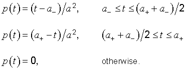
Additional guidance on evaluating uncertainty components, mainly of a practical nature, may be found in Annex F.
4.1.1 In most cases, a measurand Y is not measured directly, but is determined from N other quantities X1, X2, ..., XN through a functional relationship f:
NOTE 1 For economy of notation, in this Guide the same symbol is used for the physical quantity (the measurand) and for the random variable (see 4.2.1) that represents the possible outcome of an observation of that quantity. When it is stated that Xi has a particular probability distribution, the symbol is used in the latter sense; it is assumed that the physical quantity itself can be characterized by an essentially unique value (see 1.2 and 3.1.3).
NOTE 2 In a series of observations, the kth observed value of Xi is denoted by Xi,k; hence if R denotes the resistance of a resistor, the kth observed value of the resistance is denoted by Rk.
NOTE 3 The estimate of Xi (strictly speaking, of its expectation) is denoted by xi.
EXAMPLE If a potential difference V is applied to the terminals of a temperature-dependent resistor that has a resistance R0 at the defined temperature t0 and a linear temperature coefficient of resistance α, the power P (the measurand) dissipated by the resistor at the temperature t depends on V, R0, α, and t according to

NOTE Other methods of measuring P would be modelled by different mathematical expressions.
4.1.2 The input quantities X1, X2, ..., XN upon which the output quantity Y depends may themselves be viewed as measurands and may themselves depend on other quantities, including corrections and correction factors for systematic effects, thereby leading to a complicated functional relationship f that may never be written down explicitly. Further, f may be determined experimentally (see 5.1.4) or exist only as an algorithm that must be evaluated numerically. The function f as it appears in this Guide is to be interpreted in this broader context, in particular as that function which contains every quantity, including all corrections and correction factors, that can contribute a significant component of uncertainty to the measurement result.
Thus, if data indicate that f does not model the measurement to the degree imposed by the required accuracy of the measurement result, additional input quantities must be included in f to eliminate the inadequacy (see 3.4.2). This may require introducing an input quantity to reflect incomplete knowledge of a phenomenon that affects the measurand. In the example of 4.1.1, additional input quantities might be needed to account for a known nonuniform temperature distribution across the resistor, a possible nonlinear temperature coefficient of resistance, or a possible dependence of resistance on barometric pressure.
NOTE Nonetheless, Equation (1) may be as elementary as Y = X1 − X2. This expression models, for example, the comparison of two determinations of the same quantity X.
4.1.3 The set of input quantities X1, X2, ..., XN may be categorized as:
4.1.4 An estimate of the measurand Y, denoted by y, is obtained from Equation (1) using input estimates x1, x2, ..., xN for the values of the N quantities X1, X2, ..., XN, Thus the output estimate y, which is the result of the measurement, is given by

NOTE In some cases, the estimate y may be obtained from

That is, y is taken as the arithmetic mean or average (see 4.2.1) of n independent determinations Yk of Y, each determination having the same uncertainty and each being based on a complete set of observed values of the N input quantities Xi obtained at the same time. This way of averaging, rather than y = f(X‾‾‾1, X‾‾‾2, ..., X‾‾‾N), where

is the arithmetic mean of the individual observations Xi,k, may be preferable when f is a nonlinear function of the input quantities X1, X2, ..., XN, but the two approaches are identical if f is a linear function of the Xi (see H.2 and H.4).
4.1.5 The estimated standard deviation associated with the output estimate or measurement result y, termed combined standard uncertainty and denoted by uc(y), is determined from the estimated standard deviation associated with each input estimate xi, termed standard uncertainty and denoted by u(xi) (see 3.3.5 and 3.3.6).
4.1.6 Each input estimate xi and its associated standard uncertainty u(xi) are obtained from a distribution of possible values of the input quantity Xi. This probability distribution may be frequency based, that is, based on a series of observations Xi,k of Xi, or it may be an a priori distribution. Type A evaluations of standard uncertainty components are founded on frequency distributions while Type B evaluations are founded on a priori distributions. It must be recognized that in both cases the distributions are models that are used to represent the state of our knowledge.
4.2.1 In most cases, the best available estimate of the expectation or expected value μq of a quantity q that varies randomly [a random variable (C.2.2)], and for which n independent observations qk have been obtained under the same conditions of measurement (see B.2.15), is the arithmetic mean or average q‾‾ (C.2.19) of the n observations:

Thus, for an input quantity Xi estimated from n independent repeated observations Xi,k, the arithmetic mean X‾‾‾i obtained from Equation (3) is used as the input estimate xi in Equation (2) to determine the measurement result y; that is, xi = X‾‾‾i. Those input estimates not evaluated from repeated observations must be obtained by other methods, such as those indicated in the second category of 4.1.3.
4.2.2 The individual observations qk differ in value because of random variations in the influence quantities, or random effects (see 3.2.2). The experimental variance of the observations, which estimates the variance σ2 of the probability distribution of q, is given by
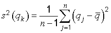
This estimate of variance and its positive square root s(qk), termed the experimental standard deviation (B.2.17), characterize the variability of the observed values qk, or more specifically, their dispersion about their mean q‾‾.
4.2.3 The best estimate of
σ2(q‾‾
) = σ2
⁄
n, the variance of the mean, is given by
The experimental variance of the mean
s2(q‾‾)
and the experimental standard deviation of the mean
s(q‾‾)
(B.2.17, Note 2), equal to the positive square root of
s2(q‾‾),
quantify how well
q‾‾
estimates the expectation
μq
of
q,
and either may be used as a measure of the uncertainty of
q‾‾.
Thus, for an input quantity
Xi
determined from
n
independent repeated observations
Xi,k,
the standard uncertainty
u(xi)
of its estimate
xi = X‾‾‾i
is
u(xi) = s(X‾‾‾i),
with
s2(X‾‾‾i)
calculated according to Equation (5). For convenience,
u2(xi) = s2(X‾‾‾i)
and
u(xi) = s(X‾‾‾i)
are sometimes called a Type A variance and a Type A standard uncertainty, respectively.
NOTE 1 The number of observations
n
should be large enough to ensure that
q‾‾
provides a reliable estimate of the expectation
μq
of the random variable
q
and that
s2(q‾‾)
provides a reliable estimate of the variance
σ2(q‾‾) = σ2⁄n
(see 4.3.2, note). The difference between
s2(q‾‾)
and
σ2(q‾‾)
must be considered when one constructs confidence intervals (see 6.2.2). In this case, if the probability
distribution of
q
is a normal distribution (see 4.3.4), the difference is taken into account through the
t‑distribution (see G.3.2).
NOTE 2 Although the variance
s2(q‾‾)
is the more fundamental quantity, the standard deviation
s(q‾‾)
is more convenient in practice because it has the same dimension as
q
and a more easily comprehended value than that of the variance.
4.2.4 For a well‑characterized measurement under statistical control, a combined or pooled
estimate of variance
s2p
(or a pooled experimental standard deviation
sp)
that characterizes the measurement may be available. In such cases, when the value of a measurand
q
is determined from
n
independent observations, the experimental variance of the arithmetic mean
q‾‾
of the observations is estimated better by
s2p
⁄n
than by
s2(qk)
⁄n
and the standard uncertainty is
u = sp
⁄
√n‾‾.
(See also the Note to H.3.6.)
4.2.5 Often an estimate
xi
of an input quantity
Xi
is obtained from a curve that has been fitted to experimental data by the method of least squares. The estimated variances
and resulting standard uncertainties of the fitted parameters characterizing the curve and of any predicted points can
usually be calculated by well-known statistical procedures (see H.3 and Reference
[8]).
4.2.6 The degrees of freedom (C.2.31)
vi
of
u(xi)
(see G.3), equal to
n − 1
in the simple case where
xi = X‾‾‾i
and
u(xi) = s(X‾‾‾i)
are calculated from
n
independent observations as in 4.2.1 and 4.2.3, should always be given when
Type A evaluations of uncertainty components are documented.
4.2.7 If the random variations in the observations of an input quantity are correlated, for example,
in time, the mean and experimental standard deviation of the mean as given in 4.2.1 and
4.2.3 may be inappropriate estimators (C.2.25) of the desired
statistics (C.2.23). In such cases, the observations should be analysed by statistical
methods specially designed to treat a series of correlated, randomly‑varying measurements.
NOTE Such specialized methods are used to treat measurements of frequency standards. However, it is
possible that as one goes from short‑term measurements to long‑term measurements of other metrological
quantities, the assumption of uncorrelated random variations may no longer be valid and the specialized methods could be
used to treat these measurements as well. (See Reference [9], for example, for a detailed
discussion of the Allan variance.)
4.2.8 The discussion of Type A evaluation of standard uncertainty in 4.2.1 to
4.2.7 is not meant to be exhaustive; there are many situations, some rather complex, that can
be treated by statistical methods. An important example is the use of calibration designs, often based on the method of least
squares, to evaluate the uncertainties arising from both short‑ and long‑term random variations in the results of
comparisons of material artefacts of unknown values, such as gauge blocks and standards of mass, with reference standards of
known values. In such comparatively simple measurement situations, components of uncertainty can frequently be evaluated by
the statistical analysis of data obtained from designs consisting of nested sequences of measurements of the measurand for a
number of different values of the quantities upon which it depends — a so‑called analysis of variance (see
H.5).
NOTE At lower levels of the calibration chain, where reference standards are often assumed to be exactly
known because they have been calibrated by a national or primary standards laboratory, the uncertainty of a calibration
result may be a single Type A standard uncertainty evaluated from the pooled experimental standard deviation that
characterizes the measurement.
4.3.1 For an estimate
xi
of an input quantity
Xi
that has not been obtained from repeated observations, the associated estimated variance
u2(xi)
or the standard uncertainty
u(xi)
is evaluated by scientific judgement based on all of the available information on the possible variability of
Xi.
The pool of information may include
For convenience,
u2(xi)
and
u(xi)
evaluated in this way are sometimes called a Type B variance and a Type B standard uncertainty,
respectively.
NOTE When
xi
is obtained from an a priori distribution, the associated variance is appropriately written as
u2(Xi),
but for simplicity,
u2(xi)
and
u(xi)
are used throughout this Guide.
4.3.2 The proper use of the pool of available information for a Type B evaluation of standard
uncertainty calls for insight based on experience and general knowledge, and is a skill that can be learned with practice. It
should be recognized that a Type B evaluation of standard uncertainty can be as reliable as a Type A evaluation,
especially in a measurement situation where a Type A evaluation is based on a comparatively small number of
statistically independent observations.
NOTE If the probability distribution of
q
in Note 1 to 4.2.3
is normal, then
σ[s(q‾‾)]
⁄
σ(q‾‾),
the standard deviation of
s(q‾‾)
relative to
σ(q‾‾),
is approximately
[2(n − 1)]−1/2.
Thus, taking
σ[s(q‾‾)]
as the uncertainty of
s(q‾‾),
for
n = 10
observations, the relative uncertainty in
s(q‾‾)
is 24 percent, while for
n = 50
observations it is 10 percent. (Additional values are given in Table E.l in
Annex E.)
4.3.3 If the estimate
xi
is taken from a manufacturer's specification, calibration certificate, handbook, or other source and its quoted uncertainty
is stated to be a particular multiple of a standard deviation, the standard uncertainty
u(xi)
is simply the quoted value divided by the multiplier, and the estimated variance
u2(xi)
is the square of that quotient.
EXAMPLE A calibration certificate states that the mass of a stainless steel mass standard
mS
of nominal value one kilogram is
1 000,000 325 g
and that “the uncertainty of this value is
240 µg
at the three standard deviation level”. The standard uncertainty of the mass standard is then simply
u(mS) = (240 µg)
⁄3 = 80 µg.
This corresponds to a relative standard uncertainty
u(mS)
⁄mS
of
80 ×10−9
(see 5.1.6). The estimated variance is
u2(mS) = (80 µg)2 = 6,4 × 10⁻⁹ g2.
NOTE In many cases, little or no information is provided about the individual components from which the
quoted uncertainty has been obtained. This is generally unimportant for expressing uncertainty according to the practices
of this Guide since all standard uncertainties are treated in the same way when the combined standard uncertainty
of a measurement result is calculated (see Clause 5).
4.3.4 The quoted uncertainty of
xi
is not necessarily given as a multiple of a standard deviation as in 4.3.3. Instead, one may find it
stated that the quoted uncertainty defines an interval having a 90, 95, or 99 percent level of confidence (see
6.2.2). Unless otherwise indicated, one may assume that a normal distribution
(C.2.14) was used to calculate the quoted uncertainty, and recover
the standard uncertainty of
xi
by dividing the quoted uncertainty by the appropriate factor for the normal distribution. The factors corresponding to the
above three levels of confidence are 1,64; 1,96; and 2,58 (see also Table G.1 in
Annex G).
NOTE There would be no need for such an assumption if the uncertainty had been given in accordance with
the recommendations of this Guide regarding the reporting of uncertainty, which stress that the coverage factor
used is always to be given (see 7.2.3).
EXAMPLE A calibration certificate states that the resistance of a standard resistor
RS
of nominal value ten ohms is
10,000 742 Ω ± 129 µΩ
at
23 °C
and that “the quoted uncertainty of
129 µΩ
defines an interval having a level of confidence of 99 percent”.
The standard uncertainty of the resistor may be taken as
u(RS) = (129 µΩ)
⁄2,58 = 50 µΩ,
which corresponds to a relative standard uncertainty
u(RS)
⁄
RS
of
5,0 × 10⁻⁶
(see 5.1.6). The estimated variance is
u2(RS) = (50 µΩ)2 = 2,5 × 10⁻⁹ Ω2.
4.3.5 Consider the case where, based on the available information, one can state that “there is a
fifty‑fifty chance that the value of the input quantity
Xi
lies in the interval
a−
to
a+”
(in other words, the probability that
Xi
lies within this interval is 0,5 or 50 percent). If it can be assumed that the distribution of possible values of
Xi
is approximately normal, then the best estimate
xi
of
Xi
can be taken to be the midpoint of the interval. Further, if the half‑width of the interval is denoted by
a = (a+ − a−)
⁄2,
one can take
u(xi) = 1,48a,
because for a normal distribution with expectation
μ
and standard deviation
σ
the interval
μ ± σ
⁄1,48
encompasses approximately 50 percent of the distribution.
EXAMPLE A machinist determining the dimensions of a part estimates that its length lies, with probability
0,5
in the interval
10,07 mm
to
10,15 mm,
and reports that
l = (10,11 ± 0,04) mm,
meaning that
± 0,04 mm
defines an interval having a level of confidence of 50 percent. Then
a = 0,04 mm,
and if one assumes a normal distribution for the possible values of
l,
the standard uncertainty of the length is
u(l) = 1,48 × 0,04 mm ≈ 0,06 mm
and the estimated variance is u2(l) = (1,48 × 0,04 mm)2 = 3,5 × 10⁻³ mm2.
4.3.6 Consider a case similar to that of 4.3.5 but where, based on the
available information, one can state that “there is about a two out of three chance that the value of
Xi
lies in the interval
a−
to
a+”
(in other words, the probability that
Xi
lies within this interval is about 0,67). One can then reasonably take
u(xi) = a.
because for a normal distribution with expectation
μ
and standard deviation
σ
the interval
μ ± σ
encompasses about 68,3 percent of the distribution.
NOTE It would give the value of
u(xi)
considerably more significance than is obviously warranted if one were to use the actual normal deviate
0,96742
corresponding to probability
p = 2
⁄3,
that is, if one were to write
u(xi) = a⁄
0,96742 = 1,033a.
4.3.7 In other cases, it may be possible to estimate only bounds (upper and lower limits) for
Xi,
in particular, to state that “the probability that the value of
Xi,
lies within the interval
a−
to
a+
for all practical purposes is equal to one and the probability that
Xi
lies outside this interval is essentially zero”. If there is no speciflc knowledge about the possible values of
Xi
within the interval, one can only assume that it is equally probable for
Xi
to lie anywhere within it (a uniform or rectangular distribution of possible values — see
4.4.5 and Figure 2 a). Then
xi,
the expectation or expected value of
Xi,
is the midpoint of the interval,
xi = (a− + a+)
⁄2,
with associated variance
If the difference between the bounds,
a+ − a−,
is denoted by
2a,
then Equation (6) becomes
NOTE When a component of uncertainty determined in this manner contributes significantly to the
uncertainty of a measurement result, it is prudent to obtain additional data for its further evaluation.
EXAMPLE 1 A handbook gives the value of the coefficient of linear thermal expansion of pure copper
at
20 °C,
α20(Cu),
as
16,52 × 10⁻⁶ °C−1
and simply states that “the error in this value should not exceed
0,40 × 10⁻⁶ °C−1”.
Based on this limited information, it is not unreasonable to assume that the value of
α20(Cu)
lies with equal probability in the interval
16,12 × 10⁻⁶ °C−1
to
16,92 × 10⁻⁶ °C−1,
and that it is very unlikely that
α20(Cu)
lies outside this interval. The variance of this symmetric rectangular distribution of possible values of
α20(Cu)
of half‑width
a = 0,40 × 10⁻⁶ °C−1
is then, from Equation (7),
u2(α20) = (0,40 ×10⁻⁶
°C−1)2
⁄3 = 53,3 × 10⁻¹⁵ °C−2,
and the standard uncertainty is
u(α20) = (0,40 × 10⁻⁶
°C−1)⁄
√3‾‾ = 0,23 × 10⁻⁶ °C−1.
EXAMPLE 2 A manufacturer's specifications for a digital voltmeter state that “between one and two
years after the instrument is calibrated, its accuracy on the
1 V
range is
14 × 10−6
times the reading plus
2 × 10⁻⁶
times the range”. Consider that the instrument is used 20 months after calibration to measure on its
1 V
range a potential difference
V,
and the arithmetic mean of a number of independent repeated observations of
V
is found to be
V‾‾‾ = 0,928 571 V
with a Type A standard uncertainty
u(V‾‾‾) = 12 µV.
One can obtain the standard uncertainty associated with the manufacturer's specifications from a Type B evaluation
by assuming that the stated accuracy provides symmetric bounds to an additive correction to
V‾‾‾,
ΔV‾‾‾,
of expectation equal to zero and with equal probability of lying anywhere within the bounds. The half‑width
a
of the symmetric rectangular distribution of possible values of
ΔV‾‾‾
is then
a = (14 × 10−6) ×
(0,928 571 V) + (2 × 10−6) ×
(1 V) = 15 µV,
and from Equation (7),
u2(ΔV‾‾‾) = 75 µV2
and
u(ΔV‾‾‾) = 8,7 µV.
The estimate of the value of the measurand
V,
for simplicity denoted by the same symbol
V,
is given by
V = V‾‾‾ + ΔV‾‾‾ = 0,928 571 V.
One can obtain the combined standard uncertainty of this estimate by combining the
12 µV
Type A standard uncertainty of
V‾‾‾
with the
8,7 µV
Type B standard uncertainty of
ΔV‾‾‾.
The general method for combining standard uncertainty components is given in Clause 5, with
this particular example treated in 5.1.5.
4.3.8 In 4.3.7, the upper and lower bounds
a+
and
a−
for the input quantity
Xi
may not be symmetric with respect to its best estimate
xi;
more specifically, if the lower bound is written as
a− = xi − b−
and the upper bound as
a+ = xi − b+,
then
b− ≠ b+.
Since in this case
xi
(assumed to be the expectation of
Xi)
is not at the centre of the interval
a−
to
a+,
the probability distribution of
Xi
cannot be uniform throughout the interval. However, there may not be enough information available to choose an appropriate
distribution; different models will lead to different expressions for the variance. In the absence of such information, the
simplest approximation is
EXAMPLE If in Example 1 of 4.3.7 the value of the coefficient is
given in the handbook as
α20(Cu) = 16,52 × 10⁻⁶ °C−1
and it is stated that “the smallest possible value is
16,40 × 10⁻⁶ °C−1
and the largest possible value is
16,92 × 10⁻⁶ °C−1”,
then
b− = 0,12 × 10⁻⁶ °C−1,
b+ = 0,40 × 10⁻⁶ °C−1,
and, from Equation (8),
u(α20) = 0,15 × 10⁻⁶ °C−1.
NOTE 1 In many practical measurement situations where the bounds are asymmetric, it may be
appropriate to apply a correction to the estimate
xi
of magnitude
(b+ − b−)
⁄2
so that the new estimate
x′i
of
Xi
is at the midpoint of the bounds:
x′i = (a− + a+)⁄2.
This reduces the situation to the case of 4.3.7, with new values
b′+ = b′− = (b+ + b−)
⁄2 = (a+ − a−)
⁄2 = a.
NOTE 2 Based on the principle of maximum entropy, the probability density function in the
asymmetric case may be shown to be
p(Xi) = A exp[− λ(Xi − xi)],
with
A = [b− exp(λb−) + b+ exp(− λb+)]−1
and
λ = {exp[λ(b− + b+)] − 1}
⁄{b− exp[λ(b− + b+)] + b+}.
This leads to the variance
u2(xi) = b+b− − (b+ − b−)⁄
λ;
for
b+ > b−,
λ > 0
and for
b+ < b−,
λ < 0.
4.3.9 In 4.3.7, because there was no specific knowledge about the possible
values of
Xi
within its estimated bounds
a−
to
a+,
one could only assume that it was equally probable for
Xi
to take any value within those bounds, with zero probability of being outside them. Such step function discontinuities in a
probability distribution are often unphysical. In many cases, it is more realistic to expect that values near the bounds are
less likely than those near the midpoint. It is then reasonable to replace the symmetric rectangular distribution with a
symmetric trapezoidal distribution having equal sloping sides (an isosceles trapezoid), a base of width
a+ − a− = 2a,
and a top of width
2aβ,
where
0 ≤ β ≤ 1.
As
β → 1,
this trapezoidal distribution approaches the rectangular distribution of 4.3.7, while for
β = 0,
it is a triangular distribution (see 4.4.6 and Figure 2 b). Assuming
such a trapezoidal distribution for
Xi,
one finds that the expectation of
Xi
is
xi = (a− + a+)⁄2
and its associated variance is
NOTE 1 For a normal distribution with expectation
μ
and standard deviation
σ,
the interval
μ ± 3σ
encompasses approximately 99,73 percent of the distribution. Thus, if the upper and lower bounds
a+
and
a−
define 99,73 percent limits rather than 100 percent limits, and
Xi
can be assumed to be approximately normally distributed rather than there being no specific knowledge about
Xi
between the bounds as in 4.3.7, then
u2(xi) = a2⁄
9.
By comparison, the variance of a symmetric rectangular distribution of half‑width
a
is
a2
⁄3
[Equation (7)] and that of a symmetric triangular distribution of half‑width
a
is
a2
⁄6
[Equation (9b)]. The magnitudes of the variances of the three distributions are surprisingly
similar in view of the large differences in the amount of information required to justify them.
NOTE 2 The trapezoidal distribution is equivalent to the convolution of two rectangular
distributions [10], one with a half‑width
a1
equal to the mean half‑width of the trapezoid,
a1 = a(1 + β)
⁄2,
the other with a half‑width
a2
equal to the mean width of one of the triangular portions of the trapezoid,
a2 = a(1 − β)
⁄2.
The variance of the distribution is
u2 = a21
⁄3 + a22
⁄3.
The convolved distribution can be interpreted as a rectangular distribution whose width
2a1
has itself an uncertainty represented by a rectangular distribution of width
2a2
and models the fact that the bounds on an input quantity are not exactly known. But even if
a2
is as large as 30 percent of
a1,
u
exceeds
a1
⁄√3‾‾
by less than 5 percent.
4.3.10 It is important not to “double‑count” uncertainty components. If a component of uncertainty
arising from a particular effect is obtained from a Type B evaluation, it should be included as an independent component
of uncertainty in the calculation of the combined standard uncertainty of the measurement result only to the extent that the
effect does not contribute to the observed variability of the observations. This is because the uncertainty due to that
portion of the effect that contributes to the observed variability is already included in the component of uncertainty
obtained from the statistical analysis of the observations.
4.3.11 The discussion of Type B evaluation of standard uncertainty in
4.3.3 to 4.3.9 is meant only to be indicative. Further, evaluations of
uncertainty should be based on quantitative data to the maximum extent possible, as emphasized in
3.4.1 and 3.4.2.
4.4.1
Figure 1 represents the estimation of the value of an input quantity
Xi
and the evaluation of the uncertainty of that estimate from the unknown distribution of possible measured values of
Xi,
or probability distribution of
Xi,
that is sampled by means of repeated observations.
4.4.2 In Figure 1 a), it is assumed that the input quantity
Xi
is a temperature
t
and that its unknown distribution is a normal distribution with expectation
μt = 100 °C
and standard deviation
σ = 1,5 °C.
Its probability density function (see C.2.14) is then
NOTE The definition of a probability density function
p(z)
requires that the relation
∫p(z)dz = 1
is satisfied.
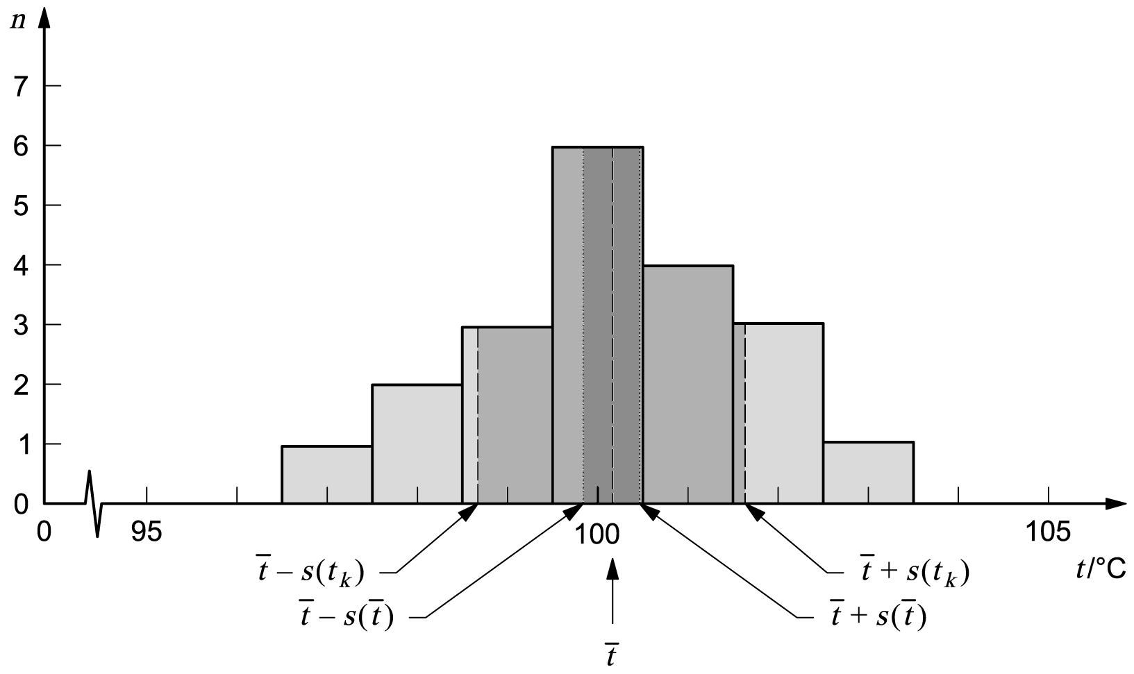
4.4.3 Figure 1 b) shows a histogram of
n = 20
repeated observations
tk
of the temperature
t
that are assumed to have been taken randomly from the distribution of Figure 1 a). To obtain
the histogram, the 20 observations or samples, whose values are given in
Table 1, are grouped into intervals
1 °C
wide. (Preparation of a histogram is, of course, not required for the statistical analysis of the data.)
The arithmetic mean or average
t‾‾
of the
n = 20
observations calculated according to Equation (3) is
t‾‾ = 100,145 °C ≈ 100,14 °C
and is assumed to be the best estimate of the expectation
μt
of
t
based on the available data. The experimental standard deviation
s(tk)
calculated from Equation (4) is
s(tk) = 1,489 °C ≈ 1,49 °C,
and the experimental standard deviation of the mean
s(t‾‾)
calculated from Equation (5), which is the standard uncertainty
u(t‾‾)
of the mean
t‾‾,
is
u(t‾‾) = s(t‾‾) = s(tk)
⁄√20‾‾‾ = 0,333 °C ≈ 0,33 °C.
(For further calculations, it is likely that all of the digits would be retained.)
NOTE Although the data in Table 1 are not implausible considering the
widespread use of high‑resolution digital electronic thermometers, they are for illustrative purposes and should
not necessarily be interpreted as describing a real measurement.
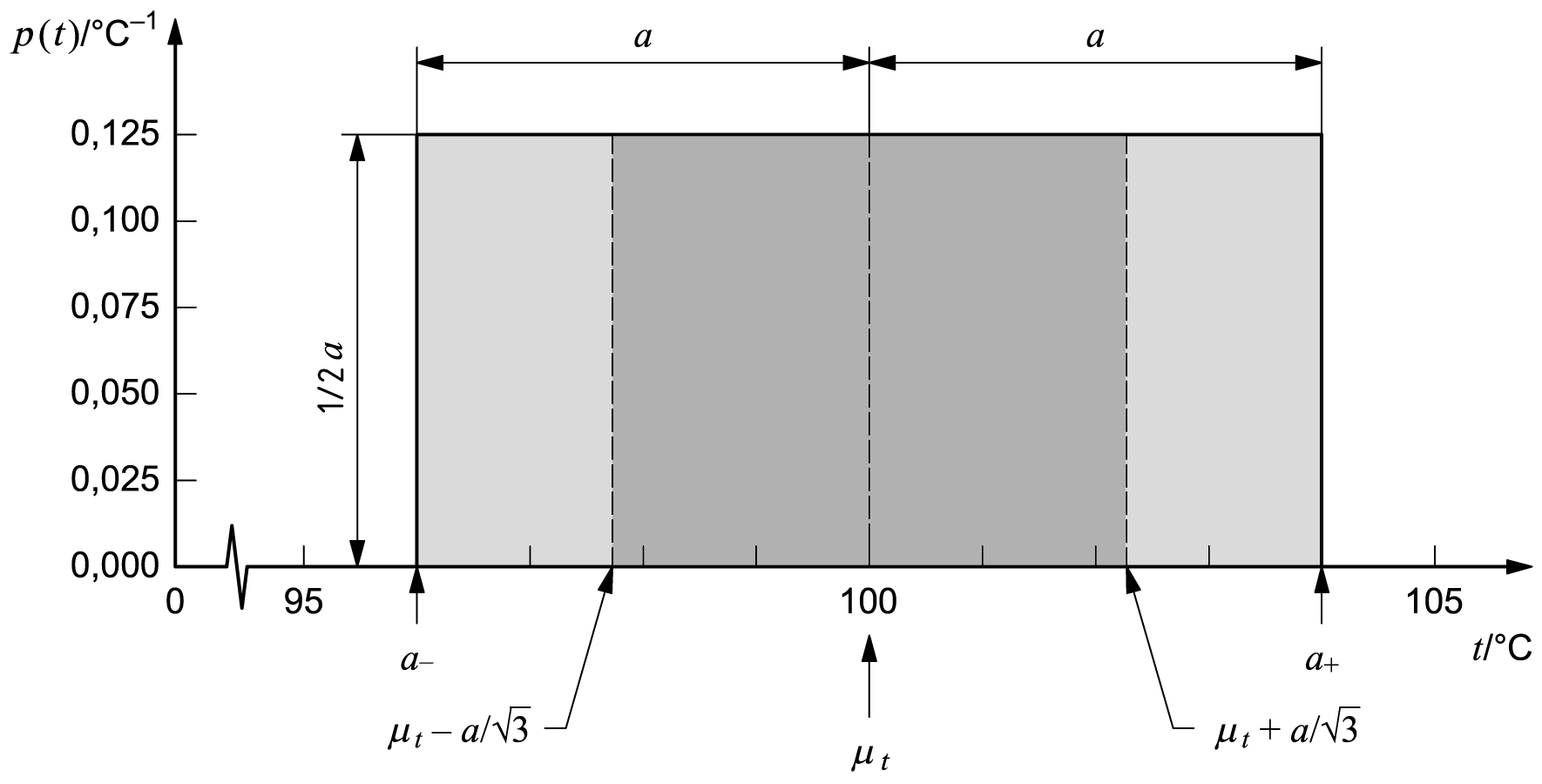
4.4.4 Figure 2 represents the estimation of the value of an
input quantity
Xi
and the evaluation of the uncertainty of that estimate from an a priori distribution of possible values of
Xi,
or probability distribution of
Xi,
based on all of the available information. For both cases shown, the input quantity is again assumed to be a temperature
t,
4.4.5 For the case illustrated in Figure 2 a), it is assumed that
little information is available about the input quantity
t
and that all one can do is suppose that
t
is described by a symmetric, rectangular a priori probability distribution of lower bound
a− = 96 °C,
upper bound
a+ = 104 °C,
and thus half‑width
a = (a+ − a−)
⁄2 = 4 °C
(see 4.3.7). The probability density function of
t
is then
As indicated in 4.3.7, the best estimate of
t
is its expectation
μt = (a+ + a−)⁄2 = 100 °C,
which follows from C.3.1. The standard uncertainty of this estimate is
u(μt) = a⁄
√3‾‾ ≈ 2,3 °C,
which follows from C.3.2 [see Equation (7)].
4.4.6 For the case illustrated in Figure 2 b), it is assumed that
the available information concerning
t
is less limited and that
t
can be described by a symmetric, triangular a priori probability distribution of the same lower bound
a− = 96 °C,
the same upper bound
a+ = 104 °C,
and thus the same half‑width
a = (a+ − a−)
⁄2 = 4 °C
as in 4.4.5 (see 4.3.9). The probability density function of
t
is then
As indicated in 4.3.9, the expectation of
t
is
μt = (a+ + a−)⁄2 = 100 °C,
which follows from C.3.1. The standard uncertainty of this estimate is
u(μt) = a⁄√6‾‾ ≈ 1,6 °C,
which follows from C.3.2 [see Equation 9 b)].
The above value,
u(μt) = 1,6 °C,
may be compared with
u(μt) = 2,3 °C
obtained in 4.4.5 from a rectangular distribution of the same
8 °C
width; with
σ = 1,5 °C
of the normal distribution of Figure 1 a) whose
− 2,58σ
to
+ 2,58σ
width, which encompasses 99 percent of the distribution, is nearly
8 °C;
and with
u(t‾‾) = 0,33 °C
obtained in 4.4.3 from 20 observations assumed to have
been taken randomly from the same normal distribution.
 (5)
(5)
4.3 Type B evaluation of standard uncertainty
 (6)
(6)
 (7)
(7)
 (8)
which is the variance of a rectangular distribution with full width
b+ + b−.
(Asymmetric distributions are also discussed in F.2.4.4 and
G.5.3.)
(8)
which is the variance of a rectangular distribution with full width
b+ + b−.
(Asymmetric distributions are also discussed in F.2.4.4 and
G.5.3.)
 (9a)
which becomes for the triangular distribution,
β = 0,
(9a)
which becomes for the triangular distribution,
β = 0,
 (9b)
(9b)
4.4 Graphical illustration of evaluating standard uncertainty

a)
b)
Figure 1 — Graphical illustration of evaluating the standard
uncertainty of an input quantity from repeated observations
 Table 1 — Twenty repeated observations of the temperature
t
grouped in
1 °C
intervals
Table 1 — Twenty repeated observations of the temperature
t
grouped in
1 °C
intervals
Interval
t1 ≤ t < t2
Temperature
t1
⁄°C
t2
⁄°C
t
⁄°C
94,5 95,5 —
95,5 96,5 —
96,5 97,5 96,90
97,5 98,5 98,18; 98,25
98,5 99,5 98,61; 99,03; 99,49
99,5 100,5 99,56; 99,74; 99,89; 100,07; 100,33; 100,42
100,5 101,5 100,68; 100,95; 101,11; 101,20
101,5 102,5 101,57; 101,84; 102,36
102,5 103,5 102,72
103,5 104,5 —
104,5 105,5 —
a)

b)
Figure 2 — Graphical illustration of evaluating the standard uncertainty
of an input quantity from an a priori distribution